Time domain reflectometry (TDR) is a method to understand the internal structure of a specimen by adding a step voltage with fast rise time on a two-terminal specimen and then observing the time variation of voltage.
This becomes a one-dimensional reader when measuring a transmission line (Note 1).
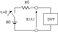
Fig.1 - Setup of TDR - E(t) Understanding the internal structure of the sample (DUT) from the waveform
The setup of TDR is very simple as shown in Fig. 1. However, a combination of a pulse generator with fast rise time and a high speed oscilloscope becomes necessary, thus this is a relatively expensive electronic measuring instrument.
R0, or the system impedance of TDR, is usually 50 Ω.
The specimen, or device under test (DUT), can be single or combinations of lumped parameter components. However, TDR is frequently used to analyze transmission lines such as high frequency transmission lines of printed circuits or high frequency cables. This is because the value of characteristic impedance that is most important in transmission lines, position and state of discontinuous section, and the propagation velocity can be measured very easily, and visual, intuitive understanding can be obtained. A simple method to use TDR using a 3C-2V (75 Ω) coaxial cable is outlined below, and we consider topics that are not written in standard literature.

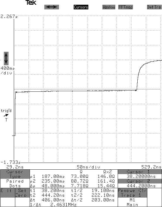
Fig.2 - TDR waveform of 3C-2Vcoaxial cable (until the fourth reflected wave returns)
Fig.2 shows the TDR waveform where an open ended 3C-2V coaxial cable is used as the DUT. In other words, the waveform of E(t) in Fig.3 is shown over the duration until the fourth reflected wave returns. The vertical axis of the TDR screen is the reflection coefficient, and the horizontal axis is time.
We must know the voltage reflection coefficients r1, r2, and r3 at the sending and receiving ends of the cable and the voltage transmission coefficients t1 and t2 at the starting end of the cable in the measuring circuit of Fig.3 to understand this TDR waveform. If you are not familiar with this subject, please read books on distributed constant circuit theory in electrical engineering.
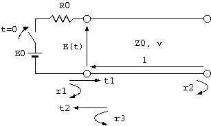
  r1 = (Z0 - R0) / (Z0 + R0) = (75 - 50) / (75 + 50) = 0.20
  r2 = (∞ - Z0) / (∞ + Z0) = 1.0
  r3 = (R0 - Z0) / (R0 + Z0) = (50 - 75) / (75 + 50) = -0.20
  t1 = 2 * Z0 / (R0 + Z0) = 2 * 75 / (50 + 75) = 1.20
  t2 = 2 * R0 / (Z0 + R0) = 2 * 50 / (75 + 50) = 0.80
Next, the transmitted wave that reached the receiving end of the cable reflects
to the original direction with reflection coefficient r2.
The transmission coefficient t2 out of the wave adds to E(t),
which becomes E(t) = r1 + t1 * r2 * t2 = 1.16.
The remaining t1 * r2 * r3 travels again to the receiving end of the cable.
The reflected wave that reached the receiving end of the terminal returns to
the sending end of the cable with reflection coefficient r2,
and the part corresponding to the transmission coefficient t2 adds to E(t),
which results in E(t) = r1 + t1 * r2 * t2 + t1 * r2 * r3 * r2 * t2 = 0.968.
At the same time, the reflected wave t1 * r2 * r3 * r2 * r3 travels to the
receiving end of the cable.
Similar reflection and transmission continues infinitely,
however, the effect of the reflected wave cannot be observed after a short
period of time because the reflection coefficient is less than 1.
Ultimately we obtain E(t) = 1 if there is no attenuation in the cable.
In reality the reflected wave becomes weaker due to attenuation,
and E(t) would converge to a value less than 1.
We notice the following after we understand this mechanism.
Defining r as the initial reflection coefficient of the sending end of the
cable, or of the connection point between R0 and DUT,
E(t) can be converted to the reflection coefficient of the DUT using
r = 2 * E(t) / E0 - 1 .
The impedance of the DUT (characteristic impedance in case of a transmission
line) through Z0 = (1 + r) / (1 - r) * R0.
The propagation velocity from the time that the reflection at the receiving
end takes to return to the sending end
The duration until the first reflected wave returns is enlarged below.
(Note 2)
Fig.4 - TDR waveform of 3C-2V coaxial cable (until the first reflected wave returns)
The vertical axis of TDR is typically given as the reflection
coefficient versus R0 and the conversion to impedance is easy, as discussed
above:
One of the main applications of TDR is to obtain the characteristic impedance
of a transmission line from the reflection coefficient.
In measurement of characteristic impedance of printed circuits,
this method is used to measure the characteristic impedance in transmission
lines.
The reflection coefficient at the left cursor in Fig.4 (black circle) is about
0.2; therefore we find that the characteristic impedance of the cable is
75 Ω. (Note 3)
We notice a mysterious fact.
The characteristic impedance of a cable is different between the sending and
receiving ends !
In case in Fig.4, the characteristic impedance is 73 Ω at the sending end
and over 80 Ω at the receiving end of the cable.
In other words, the characteristic impedance measured with TDR increases toward
the receiving end.
However, we obtain the same results when we connect the sending and receiving
ends in reverse.
Therefore, the characteristic impedance of the cable should be the same at the
sending and receiving ends.
Is there any difference between transmission lines of printed circuits and cable transmission lines?
Why does the characteristic impedance measured using
TDR increases toward the receiving end of the cable ?
This is the problem.
Note 1 - Pulse generator and oscilloscope used in TDR
The pulse generator for TDR, which is used in electronic measurements, uses
step waveforms that allow fast rise time.
The rise time is generally around 30 ps, but 7 ps rise time is achievable.
The distance resolution of TDR waveforms is on the order of 1/1000 mm.
Sampling oscilloscope techniques are usually used in the oscilloscope used in
waveform observation.
Single pulse measurement is not required, and the apparent sampling speed is
increased by carrying out many measurements of a repetitive waveform with
shifted measurement timing and by combining the results.
In contrast, TDR for detecting faults, such as breaking or shorting of long
distance cables, can have resolution on the order of 1 m.
Therefore, the rise time does not have to be very fast,
and single pulses are generally used because analysis of the reflected waveform
becomes easier.
Furthermore, use of a lower grade generator and a lower grade oscilloscope will
suffice if the time resolution does not have to be fast or you want to measure
the reflection or propagation speed of electromagnetic waves in cables that are
few 10 m long.
Similarly, devices for fault point location of cables can be built at
relatively low cost.
TDR is also used in fields such as earth sciences, agriculture, and geology in
addition to electrical engineering.
Note 2 - Measurement of attenuation using TDR
The slow rise time of reflected waves is caused by attenuation and phase
distortion of the cable, thus the half rise time of the step response can be
used to obtain the attenuation of a cable.
For details, please read
the relation between pulse rise time and cable
length on this series.
Note 3 - Measurement of propagation speed using TDR
The time until the first reflected wave returns in Fig.4 is 405 ns.
The phase velocity of the electromagnetic wave propagating in the cable is
1.98e8 using the velocity ratio of 0.66 for solid polyethylene insulated
coaxial cable,
hence we find that the cable length is 1.98e8 * 4.05e-9 / 2 = 40 m.
Conversely, we can derive the phase velocity of electromagnetic waves
propagating in a cable if we measure the length of the cable in advance.
  Z = (1 + r) / (1 - r) * R0
  Here,
	Z = Input impedance of the DUT (0 <= Z <= ∞)
	r = Reflection coefficient obtained with TDR (-1 <= r <= 1)
	R0 = Output impedance of the TDR pulse generator.
Standard TDR equipment displays the time, reflection coefficient,
and derived impedance for the point read by the cursor.
Notes
Return to Home